0
0Hello World, This is Saumya, and I am here to help you understand and implement Linear Regression in more detail and will discuss various problems we may encounter while training our model along with some techniques to solve those problems. There won't be any more programming done in this post, although, you can try it out yourself, whatever is discussed in this blog.
So now, first of all, Let's recall what we studied about Linear Regression in our previous blog. So, we first discussed about certain notations regarding to machine learning in general, then the cost function, hθ (x(i))= θ0 x0+θ1 x1. Further we discussed about training the model using the training set by running the gradient descent algorithm over it. We also discussed about the Cost Function.
Now, before we begin, I want to talk about the Cost Function in brief. Cost function, as we defined, is, J(θ)= i=1m∑( hθ(x(i))-y(i))2/ (2*m). If we define cost function, we can define it as the function, whose value is penalized by the difference between our expected value, and the actual value. Let's say, the value we obtain from hθ (x(i)) is 1000, and the actual value should have been 980. So, we'll be adding a penalty to our model of 202. And so, the task at our hand while training the model is to actually tweak the parameters in such a way, that, this penalty is the least possible value, for all the data in training set.
We'll come back to this cost function later. Before that, let's see what a polynomial regression hypothesis looks like.
If we recall, for a linear regression, we define hypothesis as hθ (x(i))= θ0 x0+θ1 x1+θ2x2, for two variables x0,x1. For the sake of simplicity, let's assume, there is only one feature, let's say radius, of the ground x0. Now, the cost will depend upon the diameter as well as area of the circle, for some crazy situation, let's assume. So, we can rewrite the hypothesis as hθ(x(i))= θ0 x0+θ1 x1+θ2x12.
So, our gradient term, that is derivative of the cost function, will become.
? J(θ)/ ?θ1= i=1m∑( hθ(x(i))-y(i))2 * x1(i)/ m
? J(θ)/ ?θ2= i=1m∑( hθ(x(i))-y(i))2 * (x1(i))2/ m
So, in short, if we substitute x12 with x2, it wouldn't make any difference to our linear regression formulas. In sum, we can say, polynomial linear regression is basically multivariate linear regression, theoretically.
Now, we can use this to add new features to our training data, generate features as a combination of two features and so on, to improve accuracy of our model. But, does higher accuracy always help? Suppose a model has 98% accuracy on training data, but when deployed, performs poorly to real world scenarios. Simultaneously, suppose a model has 90% accuracy, but it can perform better than the previous model on the real world scenario.
What might cause this issue to occur?
Is it the training data or our model selection?
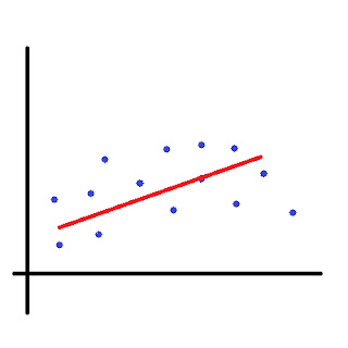
Let's see three different linear regression graphs.
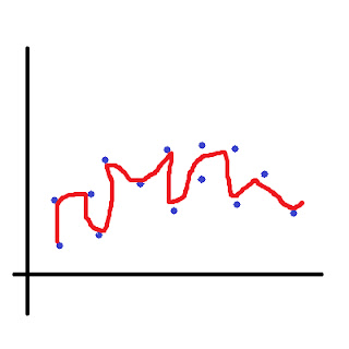
Let's say, to the above example, we added several features, so that our hypothesis becomes hθ(x(i)) = θ0 x0+θ1 x1 + θ2 x11/2+ θ3 x11/3++ θ4 x13/2…. and so on… And so our model fits in this manner now.
As, we can observe, it shows a very high accuracy rate on our training data, but it tends to consider the noise in our training data to affect our models. Basically, it is trying to fit in some anomalous data into our training model as well. This gives rise to the problem of over fitting, or high variance, since, it lets the noise model our data. Reducing the features might help us in this case.
In short, Under Fitting is low accuracy , high bias, low variance.
Whereas Over Fitting is high accuracy, low bias, high variance.
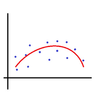
Now, since we know the solution to over-fitting, how can we reduce the features in such a way that it doesn't stay over-fitted, but it doesn't fit either. Regularization comes into play now.
So, what is regularization?
If we recall earlier, we used to penalize the model with the difference in prediction for every training example. Let's say, while training our parameter's, we want the parameters to be so small, that the noise doesn't affect our model, but not too small that it under fits the training set. So, we'll add an extra term to our cost function. which is.
J(θ)= (i=1m∑( hθ(x(i))-y(i))2/ (2*m)) + λ( j=1n∑(θ2)/(2*m) )
Where, λ is called the regularization parameter. So, what are we actually doing. We are in fact, penalizing our model for ever parameter trained, so that our model will now try to reduce not only the prediction cost, but also the parameters accordingly, as possible.
Higher the value of λ, lesser will be the value of the parameters, and Vice Versa.

The question now is, what should be the degree of the polynomial and the value of λ for an ideal model that fits our training set appropriately. Let's answer these two questions one after another.
To find the ideal degree of our polynomial, we'll first divide our actual training set into two or three parts. The new training set, which would be 60% the size of our actual set, and the rest 40% would be divided either into Cross Validation Set and Testing Set or just Cross Validation Set. Now, we'll being with a single degree and increase the degree of our polynomial, and simultaneously, train and keep track of our Cost function value.
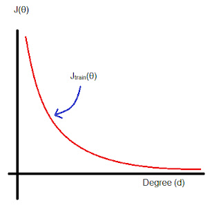
We'll notice something like this.
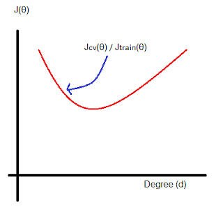
The graph will start with a very high value of cost/error function, for a very particular low degree of polynomial. But as we start increasing the degree of our polynomial function, note that the cost function starts decreasing. Note that this is done on the new training set and not on the actual training set.
Now, we'll take our cross-validation set and plot the same, cost v/s degree graph. It will turn out to be something similar to this.
So, for a low degree of polynomial, the cost will be high. And as it turns out, since the higher degree polynomial is intended to fit our training set data well, it will fit loosely to our cross-validation set. Note that, we are not supposed to train our machine using cross-validation data set. So what can we imply from this?
1 Like 0 Dislike
Follow 2 
Other Lessons for You
K-Means Clustering For Image Compression From Scratch
Hello World, This is Saumya, and I am here to help you understand and implement K-Means Clustering Algorithm from scratch without using any Machine Learning libraries. We will further use...
S
Linear Regression Without Any Libraries
I am here to help you understand and implement Linear Regression from scratch without any libraries. Here, I will implement this code in Python, but you can implement the algorithm in any other...
S
Basics Of Machine Learning
We have all been hearing recently about the term "Artificial Intelligence" recently, and how it will shape our future. Well, Machine Learning is nothing but a minor subfield of the vast field...
S
Find Machine Learning near you
Looking for Machine Learning ?
Learn from Best Tutors on UrbanPro.
Are you a Tutor or Training Institute?
Join UrbanPro Today to find students near you